How To Draw An Archimedean Spiral

Archimedean spirals are oftentimes used in the analysis of inductor coils, spiral heat exchangers, and microfluidic devices. Today, nosotros volition demonstrate how to build an Archimedean spiral using analytic equations and their derivatives to define a set of screw curves. Based on these curves, we will then create a 2nd geometry with specific thickness, extruding it to a full 3D geometry.

A Brief Introduction to Archimedean Spirals

Widely observed in nature, spirals, or helices, are utilized in many engineering designs. Every bit an electrical engineer, for instance, you may wind anterior coils in spiral patterns and pattern helical antennas. As a mechanical engineer, you may utilize spirals when designing springs, helical gears, or even the watch mechanism highlighted beneath.

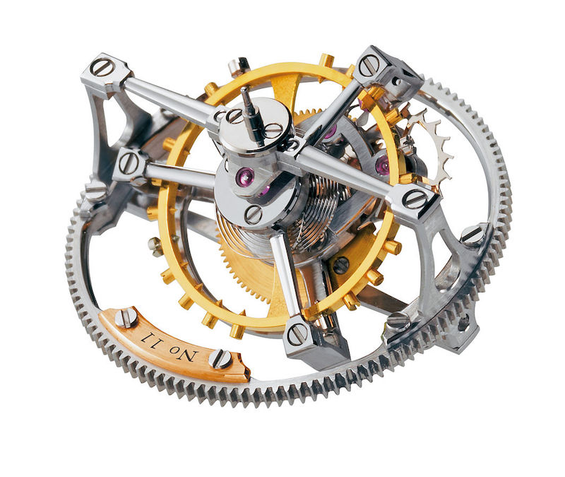
An image of a clock mechanism that features an Archimedean spiral.
An example of an Archimedean spiral used in a clock machinery. Prototype past Greubel Forsey. Licensed by CC Past-SA three.0, via Wikimedia Commons.

Here, we'll focus on a specific type of spiral, the one that is featured in the machinery shown in a higher place: an Archimedean spiral. An Archimedean spiral is a type of a screw that has a fixed distance betwixt its successive turns. This belongings enables it to exist widely used in the pattern of flat coils and springs.

We can draw an Archimedean spiral with the following equation in polar coordinates:

r=a+b\theta

where a and b are parameters that ascertain the initial radius of the screw and the distance between its successive turns, the latter of which is equal to two \pi b. Notation that an Archimedean screw is also sometimes referred to as an arithmetic spiral. This proper noun derives from the arithmetic progression of the altitude from the origin to point on the same radial.

Designing a Parameterized Archimedean Spiral Geometry

Now that we've introduced Archimedean spirals, permit's have a look at how to parameterize and create such a design for analysis in COMSOL Multiphysics.

A schematic showing the coordinates of an Archimedean spiral.
An Archimedean spiral tin can be described in both polar and Cartesian coordinates.

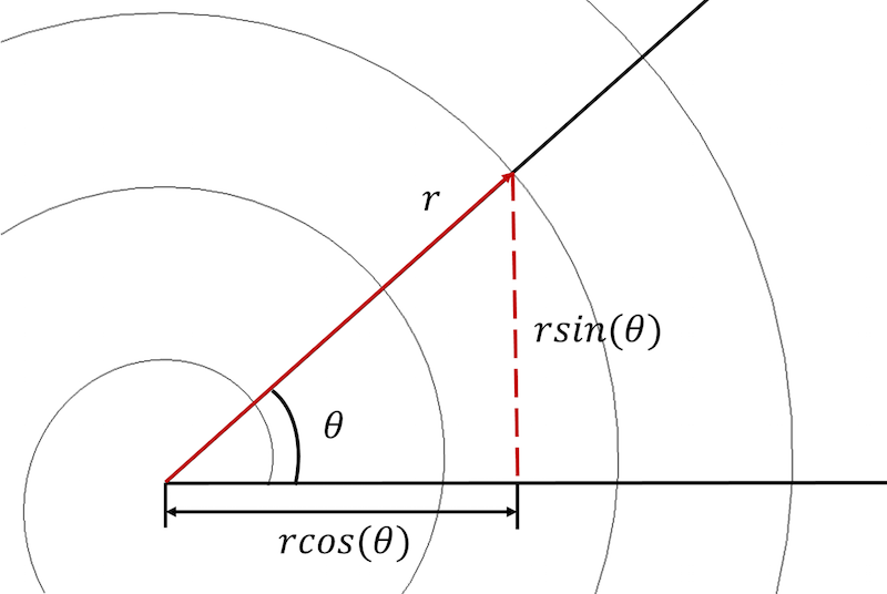
To begin, we need to convert the spiral equations from a polar to a Cartesian coordinate arrangement and express each equation in a parametric grade:

\brainstorm{align*}
x_{component}=rcos(\theta) \\
y_{component}=rsin(\theta)
\finish{align*}

This transformation allows us to rewrite the Archimedean screw'southward equation in a parametric course in the Cartesian coordinate system:

\begin{align*}
x_{component}=(a+b\theta)cos(\theta) \\
y_{component}=(a+b\theta)sin(\theta)
\end{marshal*}

In COMSOL Multiphysics, information technology is necessary to make up one's mind on the set of parameters that will ascertain the spiral geometry. These parameters are the spiral's initial radius a_{initial}, the spiral'south final radius a_{concluding}, and the desired number of turns n. The spiral growth rate b can and so exist expressed as:

b=\frac{a_{final}-a_{initial}}{2 \pi n}

Further, we need to decide on the screw's start bending theta_0 and stop bending theta_f. Let's begin with the values of theta_0=0 and theta_f=2 \pi n. With this data, nosotros are able to ascertain a set of parameters for the spiral geometry.

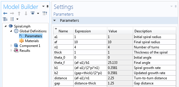
Screenshot depicting the spiral's geometric parameters.
The parameters used to build the spiral geometry.

To build this spiral, nosotros'll start with a 3D Component and create a Piece of work Plane in the Geometry branch. In the Work Plane geometry, we then add a Parametric Curve and use the parametric equations referenced above with a varying angle to draw a second version of the Archimedean spiral. These equations can be direct entered into the parametric bend's Expression field, or nosotros tin can first define each equation in a new Analytic function as:

\begin{align*}
X_{fun}=(a+bs)cos(s) \\
Y_{fun}=(a+bs)sin(s) \\
\end{align*}

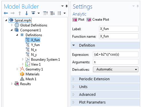
Defining an equation in the Analytic function.
The Ten-component of the Archimedean spiral equation divers in the Analytic role.

The Analytic part can be used in the expressions for the Parametric Curve. In this Parametric Curve, we vary parameter s from the initial bending of the spiral, theta_0, to the final angle of the screw, theta_f=ii \pi due north.

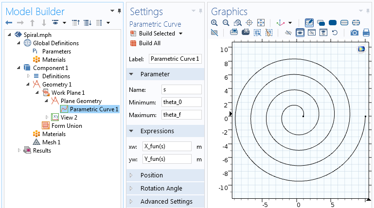
The settings for the Parametric Curve feature.

The parametric spiral equations used in the Parametric Curve feature volition consequence in a spiral represented past a curve. Let's now build upon this geometry, adding thickness to information technology in order to create a 2D solid object.

Up to this point, our spiral has been parameterized in terms of the initial radius a_{initial}, final radius a_{final}, and desired number of turns northward. Now, we must incorporate thickness as another control parameter in the screw equation.

Permit's begin with the main property of the spiral, which states that the distance betwixt the spiral turns is equal to two \pi b. This is also equivalent to \frac{a_{concluding}-a_{initial}}{due north}. To contain thickness, nosotros represent the distance between each successive plow of the spiral equally a sum of the spiral thickness and the remaining gap between turns, thick+gap.

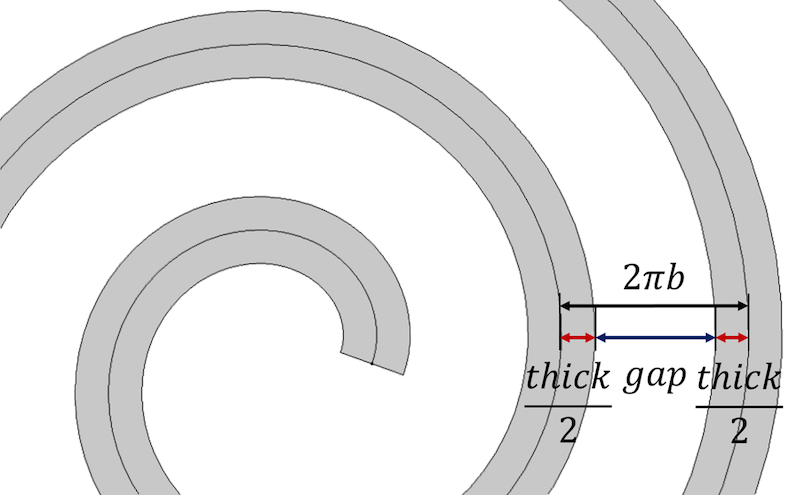
Schematic illustrating spiral thickness and gap parameters.
The distance between spirals turns is defined in terms of the spiral thickness and gap parameters.

To control thickness and obtain identical distance between the turns, the distance tin can be expressed as:

\brainstorm{align*}
distance=\frac{a_{initial}-a_{terminal}}{n} \\
gap=distance-thick
\end{marshal*}

Afterward defining thickness and expressing the gap betwixt turns in terms of thickness and constant distance between centerlines of the screw, we can rewrite the screw growth parameter in terms of thickness every bit:

\brainstorm{align*}
distance=2\pi b \\
b=\frac{gap+thick}{2\pi}
\end{marshal*}

We will also desire to express the terminal angle of the spiral in terms of its initial and concluding radii:

\begin{marshal*}
\theta_{final}=2 \pi n \\
a_{terminal}=\text{total distance}+a_{initial} \\
a_{terminal}=two \pi bn+a_{initial} \\
northward=\frac{a_{final}-a_{initial}}{2 \pi b} \\
\theta_{final}=\frac{two \pi (a_{terminal}-a_{initial})}{two \pi b} \\
\theta_{last}=\frac{a_{final}-a_{initial}}{b}
\cease{marshal*}

Want to start the spiral from an angle other than zero? If so, you will need to add together this initial angle to your concluding angle in the expression for the parameter: theta_f=\frac{a_{last}-a_{initial}}{b}+theta_0.

Duplicating the existing spiral curve twice and placing these curves with an offset of -\frac{thick}{2} and +\frac{thick}{ii} with respect to the initial spiral curve allows us to build the spiral with thickness. To position the upper and lower spirals correctly, nosotros must make certain that the offset spirals are normal to the initial spiral curve. This tin be achieved by multiplying the offset distance \pm\frac{thick}{2} by the unit of measurement vector normal to the spiral curve. The equations of the normal vectors to a curve in parametric form are:

n_x=-\frac{dy}{ds} \quad \text{and} \quad n_y=\frac{dx}{ds}

where s is the parameter used in the Parametric Curve characteristic. To become a unit normal, we need to separate these expressions by the length of the normal:

\sqrt{(dx/ds)^2+(dy/ds)^2 }

Our updated parametric equations for the Archimedean spiral with a half-thickness shift are:

\begin{align*}
x_{component}=(a+bs)cos(south)-\frac{dy/ds}{\sqrt{(dx/ds)^2+(dy/ds)^2}}\frac{thick}{ii} \\
y_{component}=(a+bs)sin(s)+\frac{dx/ds}{\sqrt{(dx/ds)^2+(dy/ds)^two}}\frac{thick}{2}
\end{align*}

Writing out these equations in the parametric curve'southward expression fields can be rather time consuming. As such, we introduce the following notation:

\begin{align*}
N_x=-\frac{dy/ds}{\sqrt{(dx/ds)^2+(dy/ds)^2}} \\
N_y=\frac{dx/ds}{\sqrt{(dx/ds)^ii+(dy/ds)^2 }}
\finish{align*}

where each N_x and N_y is defined via the Analytic function in COMSOL Multiphysics, like to how we defined X_{fun} and Y_{fun} for the start parametric curve. Within the function, we use the differentiation operator, d(f(ten),x), to take the derivative, as depicted in the post-obit screenshot.

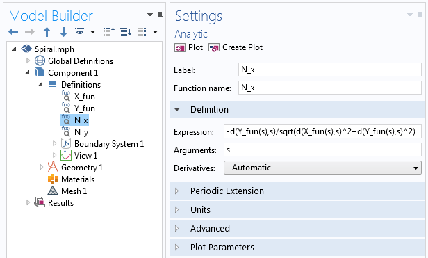
Screenshot showing examples of the derivative operator used in the Analytic function.
Examples of the derivative operator used in the Analytic part.

The functions X_{fun}, Y_{fun}, N_x, and N_y tin can and then exist used direct in the parametric bend's expressions for the bend on one side:

\begin{align*}
x_{lower}=X_{fun}(due south)+N_x(s)\frac{thick}{2} \\
y_{lower}=Y_{fun}(s)+N_y(s)\frac{thick}{2}
\finish{align*}

The functions can also be used for the curve on the other side:

\begin{align*}
x_{upper}=X_{fun}(s)-N_x(s)\frac{thick}{two} \\
y_{upper}=Y_{fun}(s)-N_y(s)\frac{thick}{2}
\end{marshal*}

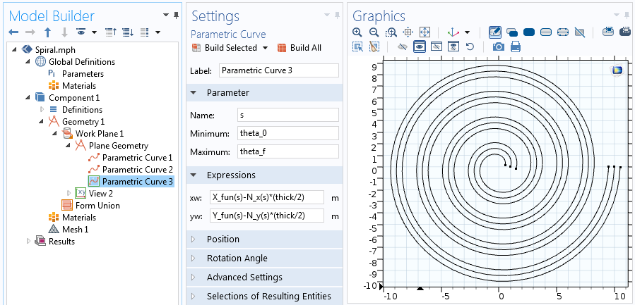
Equations for one of the offset parametric curves.
Equations for the second of the two offset parametric curves.

To join the ends of two curves, we add 2 more parametric curves using a slight modification of the equations mentioned above. For the curve that joins the eye of the spiral, nosotros have to evaluate X_{fun}, Y_{fun}, N_x, and N_y for the starting value of the angle, theta. For the curve that joins the outer side of the spiral, we have to evaluate the last value of theta. Therefore, the joining curve in the center is:

\begin{align*}
X_{fun}(theta_0)+s\cdot N_x(theta_0)\cdot\frac{thick}{2} \\
Y_{fun}(theta_0)+s\cdot N_y(theta_0)\cdot\frac{thick}{2}
\end{align*}

The outer joining curve, meanwhile, is:

\begin{align*}
X_{fun}(theta_f)+s\cdot N_x(theta_f)\cdot\frac{thick}{2} \\
Y_{fun}(theta_f)+s\cdot N_y(theta_f)\cdot\frac{thick}{ii}
\end{align*}

In both of the above equations, s goes from -1 to +1, equally shown in the screenshot below.

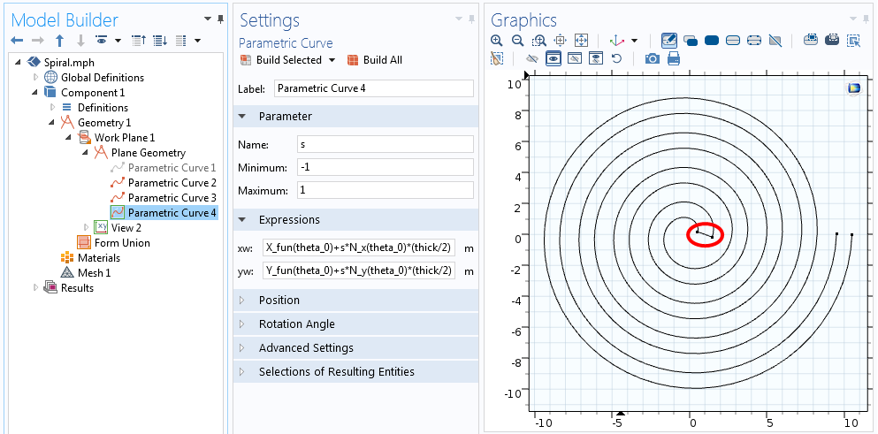
Equations for the curve joining one end of the spiral.
Equations for the curve that joins one end of the spiral.

We now have five curves that define the centerline of the screw and all four sides of the contour. We tin can disable (or even delete) the curve describing the centerline since it isn't truly necessary, leaving just the spiral outline. With the outline of our screw divers, the Convert to Solid functioning can be used to create a unmarried geometry object. This 2D spiral can finally be extruded into 3D via the Extrude performance.

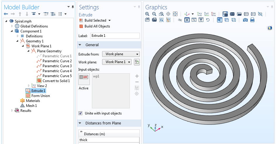
A screenshot depicting the full geometry sequence as well as the extruded 3D geometry.
The full geometry sequence and extruded 3D spiral geometry.

Endmost Remarks on Modeling Archimedean Spirals in COMSOL Multiphysics

Nosotros accept walked you through the steps of creating a fully parameterized Archimedean screw. With this screw geometry, you can modify any of the parameters and experiment with different designs, or even use them as parameters in an optimization written report. We encourage y'all to utilize this technique in your own modeling processes, advancing the analysis of your particular spiral-based engineering blueprint.

Further Resource on Designing and Analyzing Spirals

To explore further applications of simulation in the design of spiral models, try out this tutorial model: Screw Slot Antenna
Read a related user story: "Analysis of Spiral Resonator Filters"